Chapter 3 Applications
3.1 Application I: Individual-level data
The dataset used in this example is a subset of data obtained from the example datasets provided by MetaboAnalyst in the statistical meta-analysis section (Xia and Wishart, 2009). These data are from a study investigating blood-based biomarkers of adenocarcinoma and comprise 14 metabolites (N = 14) measured across 172 samples from two independent studies (K = 2). We will use `MetaHD’ for combining summary estimates obtained from these multiple metabolomic studies.
This real dataset is available in the `MetaHD’ package and can be loaded using the following command.
As explained in Section 3.1 `MetaHDInput’ function can then be used to calculate the treatment effect sizes and their associated variances and within-study covariance matrices as shown below.
##               met1      met2       met3      met4        met5         met6
## study1 -0.08509765 0.0693374 0.21205246 0.1555140 -0.07131115 -0.010729262
## study2 -0.19103975 0.1985993 0.05266387 0.3042082 -0.08507508 -0.002200277
##               met7        met8        met9      met10      met11       met12
## study1 -0.06351313  0.07239534 -0.02854481 -0.1874413 0.07670815 -0.04170964
## study2 -0.02427915 -0.08497286 -0.10315078 -0.1196099 0.07105905  0.21213759
##            met13       met14
## study1 0.3378766 -0.20944830
## study2 0.2136121 -0.03345043## met1 met2 met3 met4 met5
## met1 0.0194438538 0.0005017922 -0.0025219163 -0.002766591 0.004992537
## met2 0.0005017922 0.0161291933 0.0042058671 0.019843118 0.002535913
## met3 -0.0025219163 0.0042058671 0.0078052190 0.007030307 -0.001285968
## met4 -0.0027665912 0.0198431182 0.0070303073 0.074406890 -0.003247293
## met5 0.0049925375 0.0025359133 -0.0012859676 -0.003247293 0.007725915
## met6 0.0036952818 0.0035899796 0.0007582538 0.004244171 0.003155352
## met6 met7 met8 met9 met10
## met1 0.0036952818 0.0036649961 0.0014738763 0.002466527 0.006057970
## met2 0.0035899796 0.0023004763 0.0009291760 0.003908964 0.001622693
## met3 0.0007582538 -0.0002967142 0.0010746462 0.001839553 -0.002939468
## met4 0.0042441714 0.0033677211 0.0053704235 0.004464203 -0.001121570
## met5 0.0031553517 0.0026034856 -0.0006582206 0.002925312 0.005845677
## met6 0.0035383608 0.0025416742 0.0003542152 0.003045991 0.003098343
## met11 met12 met13 met14
## met1 0.003742686 0.0058389366 -0.017656900 0.006189749
## met2 0.006128897 0.0057661483 -0.015584915 0.002615291
## met3 0.002551313 0.0003375944 0.001663327 -0.001850528
## met4 0.005545238 0.0033374745 -0.012707585 0.001019416
## met5 0.004305489 0.0060072612 -0.020351263 0.004988612
## met6 0.003080440 0.0039539767 -0.012411644 0.003099160Now, we can carry out the multivariate meta-analysis using MetaHD as follows.
# Multivariate random-effects meta analysis
model <- MetaHD(Y = Y,
                Slist = Slist,
                method = "multi")
model$estimate
## [1] -0.1294875230 0.1390541472 0.1187040998 0.2031757519 -0.0406585464
## [6] -0.0001290338 -0.0338842144 -0.0052315949 -0.0474366927 -0.1240326912
## [11] 0.0946724585 0.1105743431 0.1909300556 -0.1084060240## [1] 0.10014867 0.08615324 0.09690759 0.25810338 0.36261181 0.99461969
## [7] 0.28079034 0.92795765 0.41512986 0.01378248 0.03066823 0.35119400
## [13] 0.01358336 0.12513848When both within and between study correlations are set to zero, MetaHD reduces to the usual random effects model analysis of individual outcomes (i.e. univariate meta-analyses). Additionally, when the between-study variances are also set to zero, then MetaHD reduces to a fixed-effects model univariate meta-analysis. We can perform univariate random-effects and univariate fixed-effects meta-analysis as follows:
K <- nrow(Y)
N <- ncol(Y)
## Create a K × N matrix of within-study variances
Smat <- matrix(0, nrow = K, ncol = N)
for (i in 1:K) {
  Smat[i, ] <- diag(Slist[[i]])
}

# Univariate random-effects meta-analysis
REmodel <- MetaHD(Y = Y,
                  Slist = Smat,
                  method = "REM")
REmodel$estimate
## [1] -0.152812325 0.137090057 0.125447557 0.236485102 -0.079158213
## [6] -0.003400283 -0.041614291 -0.005823009 -0.067093550 -0.145743652
## [11] 0.073429398 0.097637046 0.224769893 -0.115441462## [1] 0.068095503 0.117624883 0.114092805 0.198923845 0.169579668 0.878875331
## [7] 0.281592194 0.941005451 0.297222174 0.012441248 0.161809469 0.439540239
## [13] 0.009502417 0.188537212# Univariate fixed-effects meta-analysis
FEmodel <- MetaHD(Y = Y,
Slist = Smat,
method = "FEM")
FEmodel$estimate## [1] -0.152812327 0.137090057 0.119263841 0.236485102 -0.079158213
## [6] -0.003400281 -0.041614290 -0.004927685 -0.067093550 -0.145743651
## [11] 0.073429398 0.139309196 0.224769883 -0.102735148## [1] 0.068095484 0.117624861 0.036764299 0.198923825 0.169579632 0.878875296
## [7] 0.281592165 0.914730005 0.297222122 0.012441239 0.161809425 0.011347289
## [13] 0.009502382 0.034970100When missing data are available, we can use MetaHD to handle missing values by setting the argument “impute.na = TRUE”. This replaces the missing effect sizes and variances by zero and a large constant value respectively, so that the missing outcome is allocated a lower weight in the meta-analysis.
3.2 Application II: Summary-level data
In this example, we use a simulated dataset as described in Liyanage et al. (2024). We have prepared separate data frames for effect sizes and within-study covariance matrices in the simdata.1 dataset, where K = 12 (no. of studies) and N = 30 (no. of outcomes).
Now, we can carry out the meta-analysis using MetaHD as follows.
Y <- simdata.1$Y
Slist <- simdata.1$Slist

# Multivariate random-effects meta analysis
model_fastMetaHD <- MetaHD(Y = Y,
                           Slist = Slist,
                           method = "multi")
model_fastMetaHD$estimate
## [1] -0.1661335 -1.9809593 -3.7329305 -0.3676187 -1.2805349 2.2047143
## [7] -1.8351657 1.9742259 -0.7673506 -0.9405747 0.6333586 -0.8693423
## [13] 1.0744949 1.3249918 -1.2437328 1.4046179 1.1997847 0.8963671
## [19] 1.7543779 1.1155858 -0.8517850 -0.6183473 2.4147259 0.5123058
## [25] -0.8787377 -3.6860782 -1.2630573 -1.7269780 3.0223912 5.5121450If within-study correlations are not available, use only the variances and enter these values in a K x N matrix:
K <- nrow(Y)
N <- ncol(Y)
Smat <- matrix(0, nrow = K, ncol = N)
for (i in 1:K) {
  Smat[i, ] <- diag(Slist[[i]])
}

model_est.wscor<- MetaHD(Y = Y,
                         Slist = Smat,
                         method = "multi",
                         est.wscor = TRUE)
model_est.wscor$estimate
## [1] -0.07611975 -1.86284770 -3.65256960 -0.17757953 -1.23106654 2.31543281
## [7] -1.72883345 2.08240604 -0.66048927 -0.84341837 0.75958054 -0.75718192
## [13] 1.19626776 1.42655963 -1.12929204 1.49558714 1.26777701 0.94828614
## [19] 1.78974887 1.22870385 -0.77606707 -0.51324789 2.48715772 0.60812053
## [25] -0.76160149 -3.49213078 -1.12631340 -1.58589106 3.09407333 5.59067908Implementing univariate random-effects and fixed-effects meta-analysis using MetaHD:
# Univariate random-effects meta-analysis
model_random <- MetaHD(Y = Y,
                       Slist = Smat,
                       method = "REM")
model_random$estimate
## [1] 0.01698189 -1.70802518 -3.51511837 -0.03225311 -1.15230990 2.41607988
## [7] -1.61460969 2.19082837 -0.49260199 -0.79088482 0.90238451 -0.75906486
## [13] 1.26660939 1.61034022 -1.07672311 1.60752377 1.37279438 1.03478444
## [19] 1.88133989 1.29619146 -0.67308106 -0.38921814 2.65499223 0.66754678
## [25] -0.66945960 -3.49897667 -0.95282762 -1.52839939 3.20064280 5.68589161# Univariate fixed-effects meta-analysis
model_fixed <- MetaHD(Y = Y,
Slist = Smat,
method = "FEM")
model_fixed$estimate## [1] 0.01698185 -1.70802519 -3.51511838 -0.03225310 -1.15482644 2.41607988
## [7] -1.61460970 2.10129564 -0.49260199 -0.79088504 0.85325058 -0.76041187
## [13] 1.26660937 1.61034017 -1.07672316 1.60752371 1.36330932 1.03478442
## [19] 1.85911034 1.29619127 -0.67308106 -0.38921813 2.65499223 0.61682697
## [25] -0.69067483 -3.49897668 -0.95282762 -1.52839940 3.20064276 5.47152372The results obtained from different meta-analysis approaches are compared below.
true_values <- c(-0.1675687 , -1.9658875 ,-3.7501346, -0.3722893, -1.2669714,  2.1815949, -1.8274545,  2.0032794, -0.7985332 ,-0.9362461 , 0.6539242 ,-0.8254938,  1.1240729,  1.3267165, -1.2057946,1.3967554,  1.1916929 , 0.9041837,  1.7934879,  1.1444330, -0.8233060, -0.5886543,  2.4371479,  0.4882229, -0.8903039, -3.6956073, -1.2576506, -1.7221614,  3.0298406,  5.4704779)

# Create a data frame of the differences
df <- data.frame(
          Model = factor(rep(c("fastMetaHD", "fastMetaHD_est.wscor", "REM", "FEM"),each = N),
                         levels=c("fastMetaHD", "fastMetaHD_est.wscor", "REM", "FEM")),
          Difference = c(true_values - model_fastMetaHD$estimate,
                         true_values - model_est.wscor$estimate,
                         true_values - model_random$estimate,
                         true_values - model_fixed$estimate))

# Create the boxplots
ggplot(df, aes(x = Model, y = Difference, fill = Model)) +
  geom_boxplot() +
  geom_hline(yintercept = 0, linetype = "dashed") +
  scale_fill_manual(values = c("blue", "darkgreen","red","purple")) +
  labs(title = "Differences between true and estimated values for \nfastMetaHD (without divide-and-conquer), REM, and FEM",
       x = "Model",
       y = "Difference (True value - Estiamted values)")+
  theme(axis.text.x = element_text(angle = 45, hjust = 1),
        plot.title = element_text(hjust = 0.5))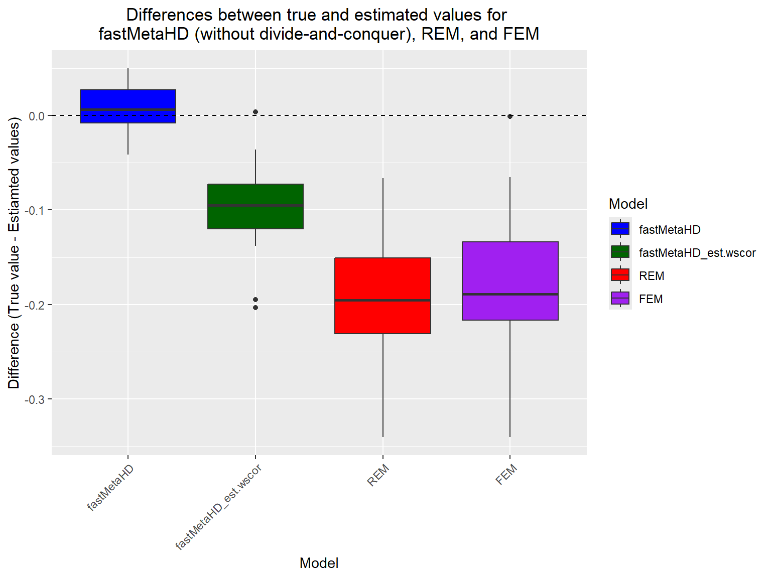
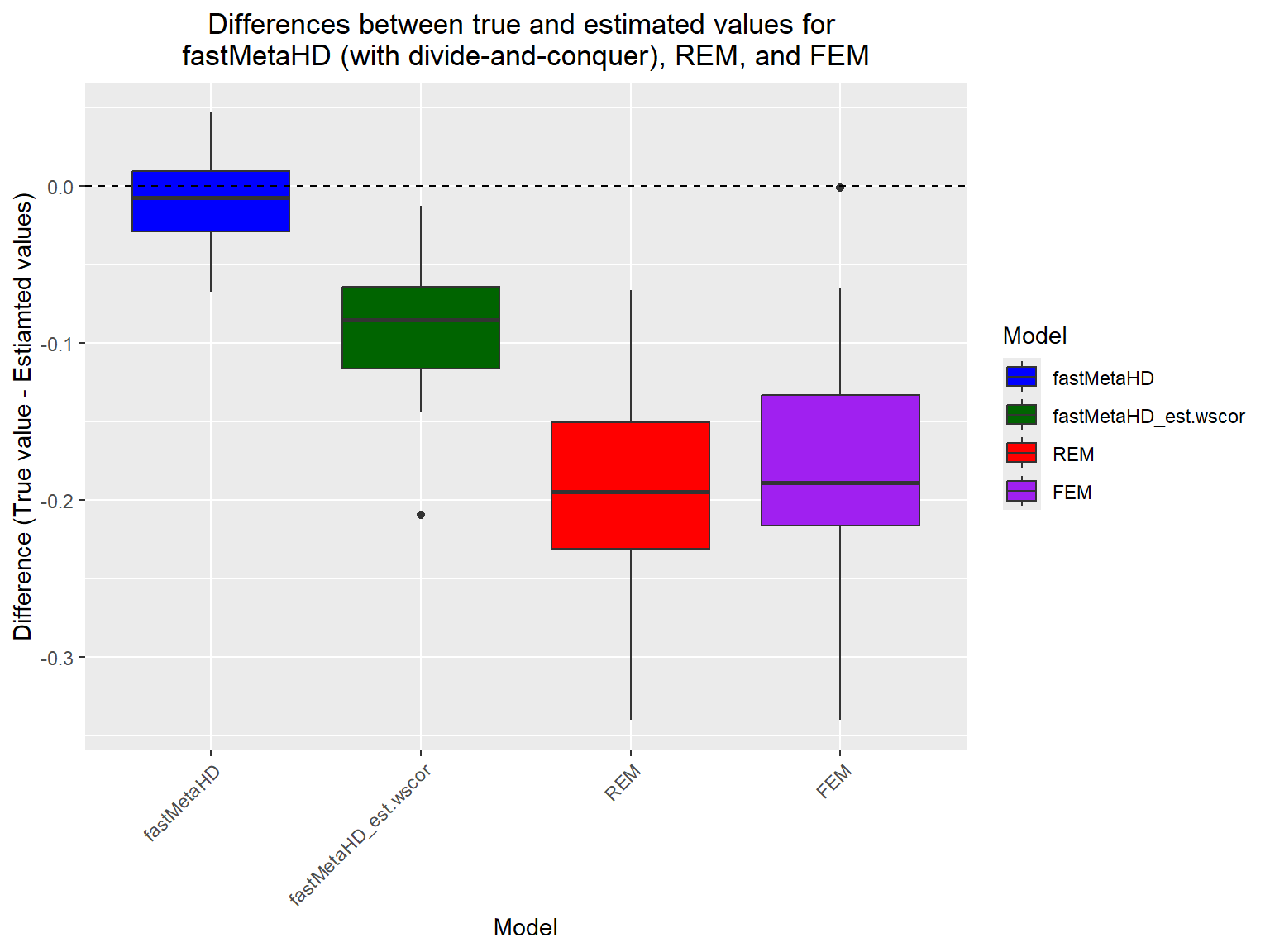
When N is large, users can implement fastMetaHD via the two-step divide-and-conquer approach. For illustrative purposes, we use the same example dataset above to demonstrate the implementation of fastMetaHD using the divide-and-conquer approach within MetaHD.
# Multivariate random-effects meta analysis via divide-and-conquer approach
model_fastMetaHD.DC <- MetaHD(Y = Y,
                              Slist = Slist,
                              method = "multi",
                              useDivideConquer = TRUE)
model_fastMetaHD.DC$estimate
## [1] -0.1578428 -1.9352834 -3.7598564 -0.3375427 -1.2563954 2.2000801
## [7] -1.8272919 2.0054146 -0.7308405 -0.9120364 0.6522972 -0.8197314
## [13] 1.1002493 1.2870452 -1.2030986 1.3970863 1.2458113 0.8949060
## [19] 1.7686248 1.1297233 -0.8696852 -0.5973989 2.4082564 0.5099695
## [25] -0.8434881 -3.6713428 -1.2027013 -1.6841568 3.0539740 5.5333904# Multivariate random-effects meta-analysis via divide-and-conquer approach when within-study correlations are unavailable
model.DC_est.wscor <- MetaHD(Y = Y,
Slist = Smat,
method = "multi",
useDivideConquer = TRUE,
est.wscor = TRUE)
model.DC_est.wscor$estimate## [1] -0.0605143 -1.8330212 -3.6727761 -0.1625469 -1.2307935 2.2921464
## [7] -1.7475588 2.1067749 -0.6624231 -0.8485452 0.7721486 -0.7472549
## [13] 1.1507732 1.4154186 -1.1329312 1.5198437 1.2748999 0.9525194
## [19] 1.8061356 1.2429361 -0.7641483 -0.5054921 2.4908075 0.5390861
## [25] -0.7555769 -3.5559144 -1.1954681 -1.5784445 3.1005675 5.5662196# Create a data frame of the differences
df <- data.frame(
Model = factor(rep(c("fastMetaHD", "fastMetaHD_est.wscor","REM", "FEM"),each = N),
levels=c("fastMetaHD", "fastMetaHD_est.wscor", "REM", "FEM")),
Difference = c(true_values - model_fastMetaHD.DC$estimate,
true_values - model.DC_est.wscor$estimate,
true_values - model_random$estimate,
true_values - model_fixed$estimate))
# Create the boxplots
ggplot(df, aes(x = Model, y = Difference, fill = Model)) +
geom_boxplot() +
geom_hline(yintercept = 0, linetype = "dashed") +
scale_fill_manual(values = c("blue", "darkgreen", "red", "purple")) +
labs(title = "Differences between true and estimated values for \nfastMetaHD (with divide-and-conquer), REM, and FEM",
x = "Model",
y = "Difference (True value - Estiamted values)")+
theme(axis.text.x = element_text(angle = 45, hjust = 1),
plot.title = element_text(hjust = 0.5))